Introduction

Among many popular graph algorithms, several algorithms allow you to find the shortest paths. Each of them solves its own problem and, accordingly, has its own application in practice. For example, the A* search algorithm can use various heuristics to find the path of the minimum cost in video games, while the Floyd — Warshell algorithm allows you to efficiently find the shortest paths between all pairs of vertices in dense graphs and can be used in the Schultz method to determine the winner of the election [1]. However, computer networks are considered to be the area where shortest path algorithms are strongly sought-for.

While developing one of our systems we faced the necessity of organizing dynamic routing in a mesh network. The infrastructure of this system was presented in the form of a set of groups where each group was a set of computing nodes within a data center. One of the aims of this system was to perform the AllReduce operation which consists in applying the reduction operation to time-varying values stored on nodes. With the help of AllReduce on each of the nodes, for example, it would be possible to have an estimation of the total amount of traffic processed in the entire network. The main goal of designing the system was to reduce the cost of data transmission between nodes of different groups.¹ An important peculiarity of the problem was that the quality of the link between the node \(a_1\) of the group \(A\) and the node \(b_1\) of the group \(B\) could significantly differ from the quality of the link between nodes \(a_2\) and \(b_2\) of the same groups because of the widespread use of ECMP routing on the Internet (the route is chosen based on the hash value from the source and recipient addresses of the packet). Therefore, we decided to implement our own dynamic routing algorithm between the nodes of the system to optimize the process of exchanging results of intermediate reduction results. We were interested in the way standard graph algorithms are used for similar problems in real distributed systems. As a result, we have done quite a deep research on the topic, and now we are ready to show you how Dijkstra’s and Bellman — Ford algorithms are used in this area.

1   Dynamic Routing

First, let us recall what the problem of dynamic routing is and what peculiarities it has.

In all modern networks, packet switching is used for data exchange. While creating a dynamic routing protocol it would be natural to want to achieve such an algorithm operation that each packet passes along some “best” route. Almost always it comes down to the problem of choosing such a neighbor through which at least one of these “best” paths to the destination node passes (here you could have noticed that the dynamic programming method is used). Such a neighbor is often called a next hop. For convenience, all current next hops are stored in the so-called routing table in which the last selected next hops are assigned to each destination object. The routing table can be updated in the background independently from the application runtime that uses communication over the network: at the time of sending a packet, it is enough to look at the routing table to understand which of the neighboring nodes is currently the most suitable for further transmission of the message.

A natural question arises: how to compare routes with each other to determine the best one? For this purpose, the concept of metric (weight, cost) of individual communication channels is introduced. Its value may depend on both their static (priority, channel bandwidth, the real cost of data transmission over it) and dynamic (RTT, the percentage of losses) parameters. In this article, we abstract from the explicit form of the metric function and assume that all nodes can calculate it at the current time. The metric of a route is defined as the sum of the metrics of links between consecutive pairs of nodes included in it.

In total, while building a routing system you need to take into account the following two features:

1. Each node of the system solves its local problem: it needs to choose a neighbor to whom it should transmit data so that it will eventually be delivered to the destination. The node \(a\) is not interested in knowing the shortest path between nodes \(b\) and \(c\) if it knows the shortest paths to each of them. Therefore, not every graph algorithm is applicable in this area. For example, the Floyd — Warshell algorithm, which finds the shortest paths between all pairs of vertices in a graph, spends additional time on this (the total complexity of this algorithm is \(O (V^3)\) ) so it makes no sense to use it in this particular case.

2. The volatile nature of the communication channels limits the set of guarantees that any dynamic routing protocol can provide. Suppose that the node \(s\) must choose one of its two neighbors \(a\) and \(b\) as the next hop to transmit the packet to the destination \(T\). Let’s assume that the route with minimum metric currently passes through the node \(a\). Within a limited time, the node \(s\) must make a final decision and start transmitting data. If we wanted to have a guarantee that the packet would pass along the route with the lowest metric then the node \(a\) should have been chosen as the next hop. Immediately after this moment, the quality of the network may change in such a way that the total metrics of all routes passing through the node \(a\) will become greater than the total metric of a route passing through \(b\). This would lead to the situation when sending proceeds in a non-optimal way. Therefore, the best that we can expect from an algorithm is a guarantee that the shortest paths will be chosen within finite time after a finite number of topological changes.

2   Dijkstra’s Algorithm and OSPF

Dijkstra’s algorithm is perhaps the most popular algorithm for finding the shortest paths in a graph. There are many resources where it is described in detail and its correctness is proved so we will only refer to one of them. Without going into details, in the algorithm, all vertices are sequentially added to the set of vertices \(U\) containing vertices to which the weights of the shortest paths are calculated. Initially, the set \(U\) is empty and all vertices are stored in the min-heap with values equal to the estimates of the lengths of the shortest paths to them. Every iteration in the algorithm consists of the relaxation of edges coming from the minimum vertex of the heap and its deletion from the heap. An edge relaxation means that the adjacent vertex is pushed up the heap if a shorter path was found through the relaxed edge.

An important aspect of this algorithm is that the node on which it is run must have a complete understanding of the network topology as a graph. In this form, it was used in the modern dynamic routing protocol OSPF [2]. In this protocol, the entire autonomous system (part of the global network in which routing is carried out) is divided into zones. Each router maintains a Link State Database (LSDB) containing information of network topology within its zone and if a change occurs it runs the Dijkstra’s algorithm with updated information. Thus, if we assume that the flooding mechanism in OSPF works correctly then the correctness of the process of building routing tables is reduced to the correctness of Dijkstra’s algorithm. You can read more about the interaction of routers in OSPF on Wikipedia.

OSPF is a prime example of the Link State approach to solving the dynamic routing problem. While using it nodes exchange information about the state of each network channel. This allows every node to have a complete picture of the current topology. It also allows nodes to relatively quickly find out if the problems occur in remote parts of the network and immediately react to them.

However, the autonomous system consists of multiple zones so an additional mechanism is needed according to which routes to external zones will be built. There is such a mechanism in OSPF: routers located on the border of the zone announce information about known routes to the external zone in the form of records with total metrics. Due to such messages routers can also build routes to objects located outside their zone. This approach is called “Distance Vector” and the Bellman — Ford algorithm is most closely related to it.

3   The Bellman — Ford Algorithm and the Distance Vector Approach

Here begins the most interesting part of the article. For further discussion, we will need a clear understanding of the classical Bellman — Ford algorithm so we will describe it by ourselves.

Let’s assume that in a weighted graph \(G = (V, E)\) we need to find the shortest paths from the vertex \(1\) to all other vertices. We will assume that \(|V| = n\). Denote by \(d_i^{(k)}\) the length of the shortest path to the vertex \(i\) found at the \(k^{\textit{th}}\) step of the algorithm. Initial values are set according to the equations:

\[\tag{1} \begin{array}{c} d_i^{(0)} = + \infty,\ i \neq 1, \\ d_1^{(0)} = 0. \end{array}\]

At each step of the algorithm, we calculate the next set of values \(d_i^{(k + 1)}\), \(i \neq 1\):

\[\tag{2} d_i^{(k + 1)} = \displaystyle \min_{j \in V,\ (j, i) \in E} \big(d_j^{(k)} + \omega(j, i)\big),\]

where \(\omega (j, i)\) is the weight of the edge \((j, i)\). Using mathematical induction it can be shown that with such an algorithm the value of \(d_i^{(k)}\) will be equal to the length of the shortest path from the vertex \(1\) to the vertex \(i\) containing no more than \(k\) edges. Thus, no later than after \(n-1\) iterations of the algorithm, we will find the shortest paths to each vertex and from some point on the values of \(d_i^{(k)}\) will stop changing. Hence, the algorithm’s complexity is easily calculated: at each iteration of the algorithm we try to relax all the edges so the total running time will be \(O (|V| \cdot |E|)\).

Let’s move on to the description of the distributed asynchronous Bellman — Ford algorithm. In the Distance Vector approach routes to various nodes are built independently of each other and the algorithm uses information from neighbors only. To reflect the changes in the problem statement we introduce new notation: without limiting generality we denote by \(D_i\) the length of the shortest path from the vertex \(i\) to the vertex \(1\). Note that this set of values is the solution of a system of equations of the form:

\[\tag{3} \begin{cases} D_i = \displaystyle \min_{j \in V,\ (i, j) \in E} \big(\omega(i, j) + D_j\big) &,\ i \neq 1 \\ D_1 = 0. \end{cases}\]

It should be noted that the sequence of sets of values \(\{d_i^{(k)}\}_{i = 1}^n\) indexed by \(k\) stabilizes to a set of values that are the solution of a system of equations similar to (3) during the operation of the standard Bellman — Ford algorithm (2). The only difference in the equations is the direction of edges which is not surprising because in one case we calculate lengths of paths from the vertex \(1\) and to it in the other. Let’s recall that the dynamic routing algorithm is run on each node of the network and each of them builds its own routing table containing estimates of the total metrics of the best routes to various destinations. In particular, each node \(i\) can maintain its own estimate \(D_i (t)\) of the value \(D_i\). We will also assume that links in our network are bidirectional: \((i, j) \in E \iff (j, i) \in E\) which means that neighbors can exchange estimates of \(D_i(t)\) and \(D_j(t)\) with each other. Thus, all nodes of the system, having received estimates from their neighbors, will be able to run an iteration of the Bellman — Ford algorithm as (3). While proving the correctness of the standard Bellman — Ford algorithm (2) we have already shown that with initial conditions (1) for fixed values of communication channels’ metrics for a finite number of iterations estimates of \(D_i (t)\) stabilize and become equal to \(D_i\). However, two problems occur. Firstly, synchronous execution of the iteration of the Bellman — Ford algorithm on all nodes of the system is difficult to implement and, moreover, impossible in the presence of failures of individual nodes. Secondly, we would like the algorithm to work with arbitrary initial conditions so that after a finite number of changes in the network it continues to build the best routes. It turns out that the algorithm continues to work correctly even with arbitrary initial states, and it is possible to perform operations on different nodes asynchronously and independently of each other.

In total, the distributed asynchronous Bellman — Ford algorithm is organized as follows. Each node \(i\) of the system for each destination at time \(t\) stores an estimate \(D_i(t)\) of the total metric \(D_i\) of the best route to it (and the corresponding next hop). The node regularly sends data about its current estimates to its neighbors. When receiving an estimate of \(D_j^i(t)\) from its neighbor \(j\) the node \(i\) updates the current estimate: \(D_i(t) := \min\big(D_i(t),\ \omega (i, j) + D_j^i (t)\big)\). If the node \(j\) is a current next hop then the current estimate is unconditionally updated: \(D_i (t): = \omega (i, j) + D_j^i (t)\). Thus, all the necessary for the algorithm data is located on neighboring nodes and it is enough to keep only the routing table in their memory. This is the Distance Vector approach to dynamic routing: a sequence of the initial node and the next hops is a route in the form of a vector the total metric of which is estimated at the initial node without maintaining the Link State Database.

In order not to overload the article with mathematics we will formulate only the idea of proving the correctness of the described algorithm. The proof takes place under the assumption that any node never stops receiving updates from its neighbors. Therefore, the mechanism for broadcasting these updates is an important part of the system but we will discuss it later. The main idea of the proof is to construct two sequences \(\{ \underline{D}_i^{(k)} \}_{k = 0}^{\infty}\) and \(\{ \overline{D}_i^{(k)} \}_{k = 0}^{\infty}\) for each node \(i\), such that

\[\underline{D}_i^{(k)} \leq \underline{D}_i^{(k + 1)} \leq D_i \leq \overline{D}_i^{(k + 1)} \leq \overline{D}_i^{(k)}.\]

These sequences are obtained from modeling the standard Bellman — Ford algorithm with different initial conditions and both of them are stabilized to \(\{ D_i \}_{i = 1}^n\). After that, it is shown that the estimates of \(D_i (t)\) on the nodes are kept between the elements of these sequences:

\[\underline{D}_i^{(k)} \leq D_i(t) \leq \overline{D}_i^{(k)}.\]

Thus, real estimates on nodes will be “clamped” between \(\underline{D}_i^{(k)}\) and \(\overline{D}_i^{(k)}\) and will eventually be equal to the total metrics of the best routes. Detailed proof can be found in the book “Data Networks” by D. Bertsekas and R. Gallagher  [3].

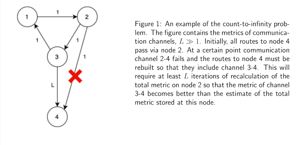
There is another, to some extent more constructive, proof in which it is shown by induction that eventually all best routes will be found starting from those with the smallest total metric and ending with the longest. However, there is a similar feature in both proofs: each of them uses induction over the set of possible values of the total metric. This may be somehow connected to a known disadvantage of the Distance Vector approach called the count-to-infinity problem (fig. 1).

4   Estimates Broadcasting

We have already mentioned that in the distributed version of the Bellman — Ford algorithm an important component is a process of broadcasting the current state of the routing table to neighbors. This can be implemented in several ways which we will briefly discuss.

The first method is called “flooding”. The node that initiates the broadcasting process tries to send data to all its neighbors. When receiving a message sent during the flooding procedure node acts the same way and so on. In the end, the information “spreads” throughout the network and if there is a working path between the initial node and some destination nodes most likely the data will reach it during the flooding process. However, this method has some disadvantages. Obviously, the data broadcasting proceeds in a non-optimal way. Moreover, if we need to send data only to adjacent nodes the method turns out to be full of redundant transmissions because flooding affects more distant nodes as well. Therefore, it is usually used in cases when it is necessary to transfer small amounts of data to all nodes of the system. For example, flooding is widely used in OSPF for broadcasting Link State Updates within the zone.

Another method is based on optimization which becomes possible thankfully to intermediate results of the dynamic routing algorithm and consists in transmitting data along the spanning tree. Initially, to do this you need to generate a message containing information about a set of destination nodes. While processing a message of this type a dictionary is created in which the keys are the current next hops in the routes to the nodes contained in the value lists. After that, the data containing the set of destination nodes is transmitted to each next hop. As a result, the broadcasting proceeds along the spanning tree that will eventually become the minimum spanning tree if the dynamic routing algorithm works correctly.

5   Techniques for Dealing with Hardware Instability

In conclusion, we will talk about how the described constructions work in real life. Namely, we will discuss several useful techniques applicable in the design of distributed systems and in the data exchange protocol for implementing the dynamic routing algorithm in particular.

5.1   Sequence Numbers

Each of the ways to implement the broadcasting operation we discussed in the last section is subject to problems of reordering and repeating messages. For clarity, we will describe examples when messages can arrive at individual nodes in an order different from the one in which they were sent.

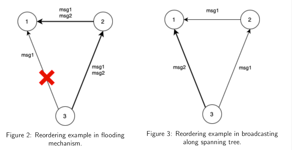
Let’s assume that in the system shown in figure 2 data broadcasting is implemented via the flooding mechanism and data transmission along the 3-2-1 route is significantly faster than through the 3-1 link. Imagine that node 3 generates two consecutive messages msg1 and msg2 for its neighbors and sends them to nodes 1 and 2, but after sending the first message link 3-1 fails and the message msg2 is not delivered over it. Node 2 after receiving messages msg1 and msg2 will send them to node 1 via link 2-1 following the flooding logic. Eventually, messages passing along the route 3-2-1 will reach node 1 earlier than the message msg1 sent over link 3-1. If the algorithm is sensitive to the order of message processing then without additional logic the last processed message will be msg1 that may lead to incorrect algorithm operation.

A similar problem may occur while using the broadcasting along the spanning tree. An example is shown in figure 3. After sending the first message msg1 the route could be rebuilt so that the second message msg2 was sent along a faster path. Thus, even in this case message reordering is possible.

In order to deal with reordering and repeating messages that will inevitably occur during flooding, it is possible to use a technique called “sequence numbers”. It involves adding a monotonically increasing over time values (versions) to messages in order to distinguish current updates from outdated ones. At the same time, each node stores a dictionary in which the keys are the identifiers of the system nodes and each value is the ordinal value of the last message received from the corresponding node. Sometimes various tags are added to the keys of this dictionary and the messages indicating which message flow they belong to. This allows engineers to reuse the data broadcasting mechanism for arbitrary purposes and not just for transmitting routing information. When a new message is received its version is compared with the corresponding value in the dictionary and if it is strictly greater the received message is processed appropriately and the version in the dictionary is updated. Otherwise, the message just received is discarded.

Message versions can be incremental. Then, in addition to solving the problem of reordering the recipient node will be able to identify gaps in the message flow and inform the sender about them. In described form this technique is used in TCP [4, p. 24]. If we do not need to track the delivery of each message the versions can be changed in such a way that the mechanism will continue to work correctly even after restarting the failed node. Since the only requirement for sequence numbers is their monotonicity you can add the number of seconds since the Epoch to the message as a version. Then the monotonicity will be preserved even throughout the launches of the same node.

5.2   TTL

Another problem that you may face while creating your own messaging protocol is loops. They can occur even in a properly designed system. For example, with frequent changes in the topology, routes can be rebuilt in such a way that some messages will pass through the same nodes an unlimited number of times. Such messages litter the network traffic and, without additional mechanisms, can cause network congestion over a long period.

To deal with infinitely “walking” messages a special integer TTL field is added to them that is equal to the maximum allowed number of hops until the message is discarded. When sending is initiated the TTL field is set to a natural number and its value is reduced by one before each transmission over the network. If the node receives a message with the TTL field equal to \(0\) it doesn’t transmit it further. However, sometimes this technique is used for other purposes. While sending a broadcast packet you can explicitly set the value of the TTL field to \(1\) so that the packet is sent only to the direct neighbors of the node.

5.3   Emergency Updates

The last technique that we will discuss is related to the optimization of dynamic routing protocols which in some cases can reduce the time of network convergence. Usually, the life cycle of a node participating in routing includes regular broadcasting of information about states of links or total metrics of routes. As long as there are no failures in the network everything works perfectly well. However, when a problem occurs one or more routes may become unavailable for data transmission and the main aim of the dynamic routing protocol is to rebuild these routes as quickly as possible. Most likely, the nodes directly interacting with the object of failure will notice the problem almost immediately but the data broadcasting timer could have triggered shortly before the problem occurred which is why other nodes will think that everything is fine until the next update is broadcasted. In addition to the count-to-infinity problem in the Distance Vector approach, this can result in a prolonged split of the entire network.

The described problem can be partially solved by introducing emergency updates which are processed according to the same algorithm as regular messages but are generated when there is a significant deterioration in routes. While using this technique it is important to make sure that all the nodes of the system for which this could be important to know about the topology changes. For example, when using the Distance Vector approach you can define the value of the difference \(\Delta_{crit}\) of the total metric that will help to detect if an emergency update is needed. The logic is as follows: if \(D_i(t_{new}) - D_i (t_{old}) \geq \Delta_{crit}\), where \(D_i (t_{new})\) is a new estimate of the total metric and \(D_i (t_{old})\) is the old one, then the corresponding emergency update is generated. After that, the information about the problem will spread along all the routes passing through the problem object without affecting those parts of the system for which it was not important.

Conclusion

This concludes the article about the adaptation of shortest path algorithms for dynamic routing problems. We formulated the engineering problem in a close to formal form, considered two main approaches to its solution: Link State and Distance Vector. We also described the distributed asynchronous Bellman — Ford algorithm and useful techniques for designing such distributed systems in conditions close to real ones.

References

[1] Markus Schulze. A new monotonic, clone-independent, reversal symmetric, andcondorcet-consistent single-winner election method. Social Choice and Welfare, 36(2):267–303, July 2010.

[2] John Moy. Ospf version 2. STD 54, RFC Editor, April 1998. http://www.rfc-editor.org/rfc/rfc2328.txt

[3] Dimitri Bertsekas and Robert Gallager. Distributed Asynchronous Bellman-FordAlgorithm, pages 404–410. Prentice-Hall, Inc., Englewood Cliffs, New Jersey07632, 1992.

[4] Jon Postel. Transmission control protocol, STD 7, RFC Editor, September 1981, https://www.rfc-editor.org/rfc/rfc793.txt

---

1. If we try to formalize the concepts of cost and quality it is easy to see that, as often happens in life, they are directly dependent — that is, generally speaking, it is impossible to simply reduce the former and increase the latter. For example, it would be possible to reduce the total amount of data transmitted between all nodes (cost) if you select one group where the reduction will take place and which will then send the result of the reduction to everyone else. However, compared to the implementation when each group exchanges data directly with each other the delay increases and the fault tolerance of the system decreases, that is, the quality decreases. Thus, in practice, it is necessary to find a balance between these goals but the specific choice is not relevant to the further presentation.↩